책에서 4장부터 14장까지 모델링의 기초를 전부 다루었기에 15장에서는 이전에서 배운 것을 바탕으로 모델링의 과정에 대해 리마인드 겸 전체적으로 설명하는 것 처럼 보입니다. 간단하게 각 챕터마다 배운 것을 요약하면 아래와 같습니다.
- [4장] 모델링에 사용될 데이터(Ames Housing) EDA
- [5장] 데이터 풀을 Training data와 Testing data로 나눠야 하는 이유와 rsample 함수 소개
- [6장] 패키지마다 모델링 인터페이스가 다른 것을 통일한 parsnip 패키지 설명과 함께 모델 구축, 적합, 예측 함수 소개
- [7장] Model Workflow 소개 (workflow, workflow_set)
- [8장] Recipes 패키지를 이용한 Feature Engineering
- [9장] yardstick 패키지를 이용한 Performance Metric
- [10장] 리샘플링 데이터를 사용해야하는 이유와 교차검증 및 붓스트랩 설명
- [11장] 리샘플링을 이용한 여러 모델의 비교 (하이퍼파라미터 튜닝 제외)
- [12장] 하이퍼 파라미터의 값을 데이터에서 직접 구하기 어려운 이유와 튜닝의 중요성 설명
- [13장] 하이퍼 파라미터 튜닝 - 그리드서치(Grid Search)와 tune_grid를 통한 평가
- [14장] 하이퍼 파라미터 튜닝 - Iterative Search(Bayesian Optimization / Simulated Annealing)
15 Screening Many Models | Tidy Modeling with R
The tidymodels framework is a collection of R packages for modeling and machine learning using tidyverse principles. This book provides a thorough introduction to how to use tidymodels, and an outline of good methodology and statistical practice for phases
www.tmwr.org
우선 본문에서처럼 다음과 같이 데이터 변형 후 Train/Test 데이터 셋으로 나누고 리샘플링 데이터를 만들어 줍니다.
(속성이 같은 데이터를 여러번 측정하였기 때문에 compressive_strength를 제외한 나머지 변수의 값들을 그룹화하였습니다.)
### 15. Screening Many Models
# >> 잘 모르는 새로운 데이터로 작업할 때 많은 모델과 전처리기를 생성해서 관찰하는게 좋을 수 있다.
# >> 많은 모델을 관찰해 좋은 소규모의 모델을 선택 후 정밀한 최적화 진행
# >> workflow set은 이런 과정을 관리하는 인터페이스를 제공

library(tidymodels)
library(tidyverse)
library(usemodels)

### Data Preparing
data(concrete, package = "modeldata")
glimpse(concrete)

concrete <-
  concrete %>%
  group_by(across(-compressive_strength)) %>%
  summarize(compressive_strength = mean(compressive_strength),
            .groups = "drop")

concrete_split <- initial_split(concrete, strata = compressive_strength, prop = 0.75)
concrete_train <- training(concrete_split)
concrete_test  <- testing(concrete_split)
concrete_folds <-
  vfold_cv(concrete_train, strata = compressive_strength)
또한 본문에서처럼 레시피와 모델은 각각 아래와 같이 생성하였습니다.
### Recipe
normalized_recipe <-
  recipe(compressive_strength ~ ., data = concrete_train) %>%
  step_normalize(all_numeric_predictors())

poly_recipe <-
  normalized_recipe %>%
  step_poly(all_numeric_predictors()) %>%
  step_interact(~all_numeric_predictors() : all_numeric_predictors())
### Modeling
library(rules)
library(baguette)
linear_model <-
linear_reg(penalty = tune(), mixture = tune()) %>%
set_engine("glmnet")
nnet_model <-
mlp(hidden_units = tune(), penalty = tune(), epochs = tune()) %>%
set_engine("nnet", MaxNWts = 2600) %>%
set_mode("regression")
mars_model <-
mars(prod_degree = tune()) %>% #<- use GCV to choose terms
set_engine("earth") %>%
set_mode("regression")
svm_rbf_model <-
svm_rbf(cost = tune(), rbf_sigma = tune()) %>%
set_engine("kernlab") %>%
set_mode("regression")
svm_poly_model <-
svm_poly(cost = tune(), degree = tune()) %>%
set_engine("kernlab") %>%
set_mode("regression")
knn_model <-
nearest_neighbor(neighbors = tune(), dist_power = tune(),
weight_func = tune()) %>%
set_engine("kknn") %>%
set_mode("regression")
cart_model <-
decision_tree(cost_complexity = tune(), min_n = tune(), tree_depth = tune()) %>%
set_engine("rpart") %>%
set_mode("regression")
bag_cart_model <-
bag_tree(cost_complexity = tune(), tree_depth = tune(), min_n = tune()) %>%
set_engine("rpart", times = 50L) %>%
set_mode("regression")
rf_model <-
rand_forest(mtry = tune(), min_n = tune(), trees = 1000) %>%
set_engine("ranger") %>%
set_mode("regression")
xgboost_model <-
boost_tree(tree_depth = tune(), learn_rate = tune(), loss_reduction = tune(),
min_n = tune(), sample_size = tune(), trees = tune()) %>%
set_engine("xgboost") %>%
set_mode("regression")
cubist_model <-
cubist_rules(committees = tune(), neighbors = tune()) %>%
set_engine("Cubist")
nnet_param <-
nnet_model %>%
extract_parameter_set_dials() %>%
update(hidden_units = hidden_units(c(1, 27)))
nnet_param %>% extract_parameter_dials("hidden_units")
챕터 7장에서 workflow sets을 만들어보았는데요. Workflow_set, Workflow_variables 함수를 사용해 3가지의 워크플로셋 객체를 만든다음 하나의 객체로 만들기 위해서 bind_rows 함수를 사용하였습니다. (각 레시피마다 적용되는 모델들이 다른지는 본문 참고)
### Create Workflow sets
# [1] wflow_id : preproc과 models의 이름을 조합하여 자동으로 생성됨
# [2] info : 식별자와 워크플로 객체가 포함된 티블
# [3] option : 워크플로 객체를 평가할 때 사용하고자 하는 인자를 포함한 공간으로
#              tune 패키지에 포함된 함수 사용시 해당 인자를 적용

normalized <- workflow_set(
  preproc = list(normalized = normalized_recipe),
  models = list(SVM_radial = svm_rbf_model, SVM_poly = svm_poly_model,
                KNN = knn_model, neural_network = nnet_model))
normalized <- normalized %>%  # tune_grid에 사용하기 위해서
  option_add(param_info = nnet_param, id = "normalized_neural_network")

model_vars <- workflow_variables(outcomes = compressive_strength,
                                 predictors = everything())
no_pre_proc <- workflow_set(
  preproc = list(simple = model_vars),
  models = list(MARS = mars_model, CART = cart_model, CART_bagged = bag_cart_model,
                  RF = rf_model, boosting = xgboost_model, Cubist = cubist_model))

with_features <- workflow_set(
  preproc = list(full_quad = poly_recipe),
  models = list(linear_reg = linear_model, KNN = knn_model))

# Combind all workflows into single object
all_workflows <-
  bind_rows(no_pre_proc, normalized, with_features) %>%
  mutate(wflow_id = str_replace(wflow_id, "(simple_)|(normalized_)", ""))
print(all_workflows)
일단 현재 다수의 워크플로 객체는 튜닝 파라미터를 가지고 있는데요. 그렇다면 바로 리샘플링 객체를 피팅하기 전에 하이퍼파라미터의 값부터 튜닝부터 해야할 것입니다. 따라서 여러개의 워크플로 객체를 가지고 있는 workflow set 객체에 각 워크플로에 함수를 따로 적용하는 workflow_map 함수를 사용하여 tune_grid를 개별적으로 적용해줍시다. (빠른 결과를 위해서 tune_race_anova를 적용해도 됩니다)
### Tuning and Evaluating the models
grid_ctrl <- control_grid( save_pred =T, save_workflow = T,
                           parallel_over = "resamples", verbose = T)

grid_results <- all_workflows %>%
  workflow_map(fn = "tune_grid", seed =1,
               resamples = concrete_folds,
               control = grid_ctrl)
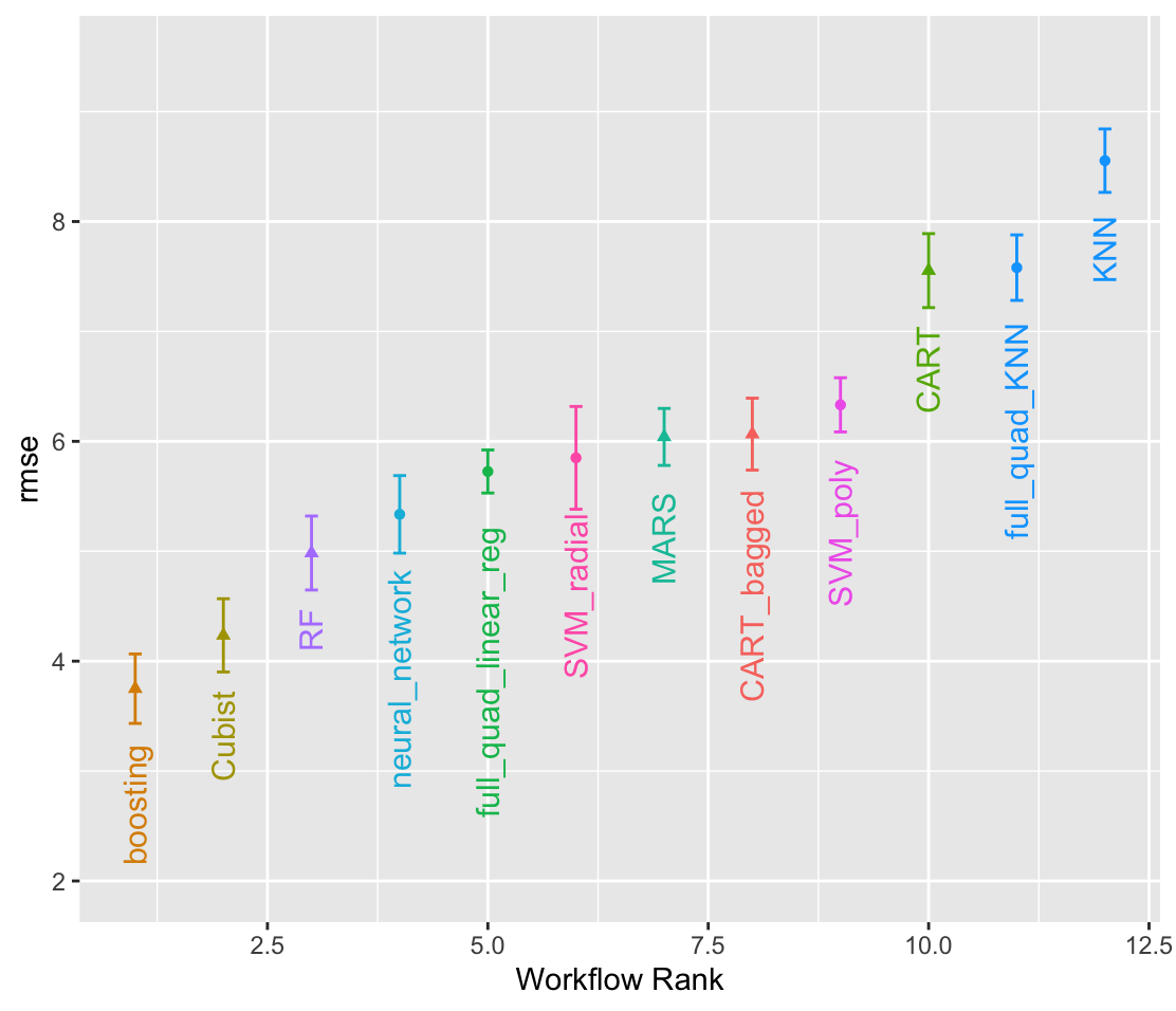
tune_grid를 개별 워크플로에 적합하면 나면 하이퍼파라미터 값에 따라 Training data를 학습하고 Validation data를 통해 성능지표를 도출합니다. 여기서는 RMSE를 기준으로 모델을 선택하며 rank_results 함수와 autoplot 함수를 통해서 모델들의 성능을 확인해 봅시다.
랭킹과 그래프 모두 최고의 성능을 내는 모델은 부스팅에서 나왔으며 rmse의 구간을 살펴보면 부스팅이 제일 뛰어나나 큐비스트 모델과 일부 구간을 공유하는 것을 볼 수 있습니다.
grid_results %>% rank_results() %>%
  filter(.metric == "rmse") %>%
  select(model, .config, rmse = mean, rank)

grid_results %>% autoplot(rank_metric = "rmse", metric = "rmse", select_best = T) +
  geom_text(aes(y = mean - 1/2, label = wflow_id), angle = 90, hjust = 1) +
  lims(y = c(2, 9.5)) +
  theme(legend.position = "noen")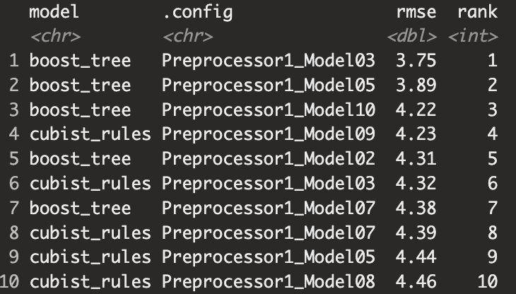
부스팅 모델이 가장 성능이 좋았으므로 Iterative Search를 통해서 하이퍼파라미터의 값을 더 좋은 결과가 나올 수 있도록 수정해줍시다. 해당 코드 실행 결과 그리드서치로 구한 최적값과 조금 차이가 있다는 것을 알 수 있습니다.
### Best Model's Iterative Search
boost_SA <- tune_sim_anneal(object = grid_results %>% extract_workflow("boosting"),
                resamples = concrete_folds,
                initial = grid_results %>% extract_workflow_set_result("boosting"),
                iter = 50, metrics = metric_set(rmse),
                control = control_sim_anneal(verbose = T))
SA_best_results <- boost_SA %>% select_best()

best_result <- grid_results %>%
  extract_workflow_set_result("boosting") %>%
  select_best(metric = "rmse")

print(best_result)
print(SA_best_results)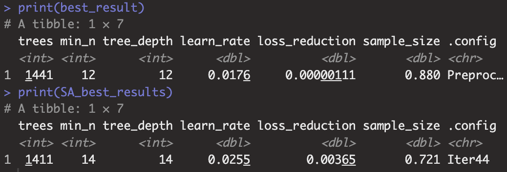
이제 튜닝 된 하이퍼파라미터 값을 가지고 최종 모델을 생성해야 합니다. 워크플로 객체가 모여있는 all_workflows나 하이퍼파라미터 튜닝이 진행된 grid_result 모두 extract_workflow 함수를 통해 전처리가와 모델이 지정된 특정 워크플로 모델을 지정할 수 있으므로 해당 객체에서 우리가 원하는 모델의 워크플로를 추출해야 합니다.
finalize_workflow 함수를 통해서 우리가 Iterative Search를 통해 찾은 값을 전달할 수 있으며 하이퍼파라미터 값이 전달된 모델을 통해서 Train data(Train + Validation, 최종모델이므로 가능한 모든 데이터 사용) 데이터를 적합하고 Test data로 모델의 성능을 평가해야 합니다. last_fit 함수를 통해 간단하게 구현할 수 있으며 최종 성능지표는 rmse 기준 4.69 정도 나오는 것을 확인할 수 있습니다.
### Finalizing
boosting_final_model <- grid_results %>%
  extract_workflow("boosting") %>%
  finalize_workflow(SA_best_results) %>%
  last_fit(split = concrete_split)

boosting_final_model %>% collect_predictions() %>%
  rmse(truth = compressive_strength, estimate = .pred)
boosting_final_model %>% collect_metrics()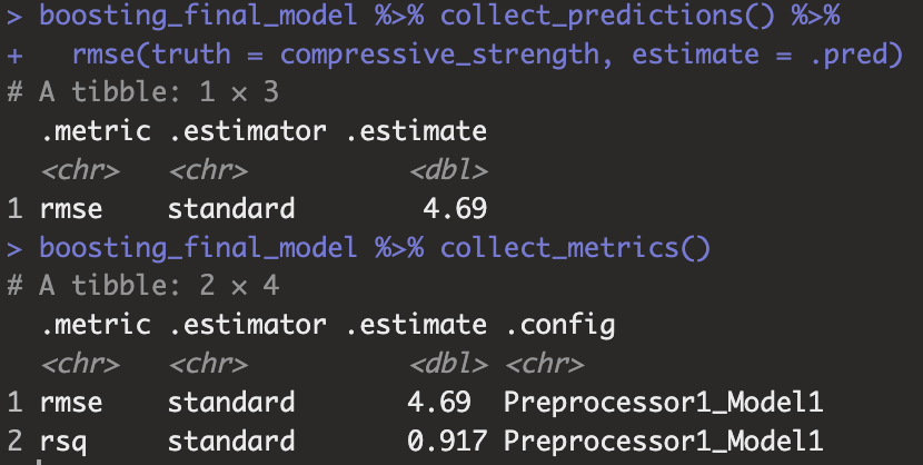
또한 마지막으로 실제값과 예측값이 얼만큼 차이가 있는지 확인해 보면 아래와 같은데, 점선에 가까울수록 모델이 예측을 잘 한것이며 저희가 적합한 모델을 보면 일부 점들을 제외하고는 대부분의 점들이 점선 근처에 모여있는 것을 확인할 수 있겠습니다.
boosting_final_model %>%
  collect_predictions() %>%
  ggplot(mapping=aes(x=compressive_strength, y=.pred)) +
  geom_abline(color="grey40", lty=2) +
  geom_point(alpha = 0.5) +
  coord_obs_pred() +
  labs(x="observed", y="predicted")
'Data Science > Modeling' 카테고리의 다른 글
| [Tidymodels] Bagging Model with IBM Churn data (2) | 2024.04.03 |
|---|---|
| [Tidy Modeling with R] 16. 차원 축소(Dimensionality Reduction) (2) | 2024.01.07 |
| [Tidy Modeling With R] 14. Iterative Search with XGBoost (2) | 2023.12.26 |
| [Tidy Modeling With R] 13. Grid Search with XGBoost (2) | 2023.12.22 |
| [Tidy Modeling with R] 12. 하이퍼파라미터 튜닝 (0) | 2023.10.11 |